Friday, June 21, 2024

Impact of Deep Learning and Applications in Biomedicine


Impact of Deep Learning and Applications in Biomedicine

Introduction

Deep learning is a new and quickly growing field of artificial intelligence. It aims to demonstrate reasoning based on a variety of information, using different Deep Neural Networks (DNNs) to detect information like images, speech, and text. Moreover, deep learning has two common features first, various layers of nonlinear computational units and second, superintending or learning of the elements introduced in each layer (Yu D [1]). In the 1980s the first deep learning systems were based on pseudo neuron or Artificial Neural Networks (ANN), and the true impact of deep learning was not evident and visible until 2006 (Fukushim, et al. [2-4]). From that time till now, deep learning has found applications and been used in diverse fields such as programmatic speech recognition, image recognition an engineering application of machine learning, the application of computational techniques to the analysis and synthesis of natural language and speech, drug making process, and bioinformatics (Cios K J, et al. [5-7]). In recent years, biomedical data has been greatly aided by the development of high-throughput technological innovations including genome sequencing, protein engineering, and clinical/medical images. Most importantly, powerful and efficient computers are needed to store, analyze and decode this large amount of biomedical information (Cios K J, et al. [5,8]).

The deep learning algorithmic systems collectively identified and enlightened these complex issues. Accordingly, the objective of this article is to bring forth an overview of deep learning methods for the local field of bioinformatics and biomedical informatics and to present some of the recent applications of deep learning in biomedicine. It is anticipated that this article will provide people an outline of deep learning and make it understandable that how it can be successfully used to examine biomedical information.

Current Metrics

Regardless of the enormous benefits of deep learning, there are still problems with its application in the biomedical field. Likewise, using background images, we show how deep learning can characterize the extent of diabetic retinopathy and attempt to identify wound or damaged area in multiple ways. In addition to high degree of accuracy and momentum, deep learning’s intelligent use of response fields gives it a big advantage in pattern recognition. Along with that, improved head-to-tail classification using deep learning also gives new ideas and throws light on characterizing and assorting pixels as injured or not. Whereas the application of deep learning to clinical/ medical images is still in the testing phase. When creating models, we want to get a lot of information, sometimes data with labels, directly in the order for classifying the pixels. Naming these medical images physically is difficult and hence necessitate seasoned professionals. Furthermore, these medical images are closely related to data security, so it is crucial to understand and protect the information. Also, biomedical information tends to be unbalanced when the amount of information in general categories is greater than the amount of information in other categories. Despite the balancing hurdles, the amount of information and data needed, and the nomenclature/ naming of biomedical information, deep learning entails and necessitates technological upgradation and innovation. In any case, discrete differences and changes in clinical images would indicate disease because they are different than the normal images. That is why, examining these images needs high resolution, fast processing and having the capacity of incorporating large memory. In addition, it is challenging to identify and discover a single evaluation metric for grouping and predicting biomedical information.

Alongside, different from other projects, it handles false trends to some extent and does not reject (many) false negatives in disease detection. In case of dealing with distinct and unalike, it is necessary to thoroughly test the model and adjust its informative quality as per the features and attributes of the data. Luckily, deeper coordinates can be accelerated in the inception modules (He K [9,10]), and higher degree of accuracy can be achieved in biomedical imaging studies (Yarlagadda D V K, et al. [11]). Also, collection of information, opinions, or work from a group of people, usually sourced via the Internet (crowdsourcing pathway) have started to lay the foundation for the collection of annotations, which could be a significant tool in the near future. Hence, these two engines will facilitate the use of deep learning in the field of biomedical informatics (Albarqouni S, et al. [12-14]).


For more Articles on: https://biomedres01.blogspot.com/

Wednesday, June 19, 2024

On Pre-Weaning Calf Weight Gain Differences: Opportunities to Improve Herd Productivity, Health and Longevity


On Pre-Weaning Calf Weight Gain Differences: Opportunities to Improve Herd Productivity, Health and Longevity

Introduction

Traditionally, dairy calves are fed milk at about 8-10% of birth body weight to increase starter feed intake and achieve early and timely weaning. This practice may reduce rearing costs but can also reduce average daily weight gain (ADG) as a result of decreased nutrient intake [1]. The growth performance and health status of dairy heifers in early stages of life have attracted much attention over the past two decades. Greater weaning weights have been observed in calves on ad libitum milk feeding regimens [2]. Such a greater pre-weaning weight gain might relate to later performance of dairy heifers [3]. Accordingly, some nutritional concepts such as enhanced or intensified milk feeding programs have been developed [4]. Under such systems, milk is fed at approximately 20% of body weight to resemble the time when calves are raised with their mothers. Recent works also support this idea that increased milk intake to gain more weight in the pre-weaning period might be translated into greater milk yield in the subsequent lactation [5]. Given the potential benefits of greater ADG in early-life; however, it seems that considerable variations exist in ADG among farms in the U.S. (the NAHMS report, 2014) and likely worldwide. Some questions come to the mind. Are the producers aware of the possible positive effects of increased pre-weaning ADG on herds’ productivity and longevity? To what extent are the scientific reports applicable to commercial circumstances? Addressing these questions may help the dairy industry establish sustainable heifer raising systems globally.

In an interview with dairy farmers and their advisors, it turned out that farmers did not receive adequate instructions for optimal feeding of young calves. This would suggest, and reflect in, undernutrition and reduced ADG in early calf life [6]. According to this interview, most of the farmers in the UK used traditional milk feeding programs despite the fact that intensified milk feeding programs have been emphasized. In addition, calf growth performance in the literature is commonly expressed in a single time period [7], while weight gain in the later pre-weaning phases (from 3-4 weeks of age up to weaning) is totally greater than that in the early pre-weaning period (the first three weeks of life). In studies investigating the pre-weaning period as two separate phases including
1. The first three weeks and
2. The rest, the results have shown large differences in ADG of calves under different milk feeding strategies (intensified vs. conventional) in early life [8,9].

It seems that plan of nutrition during the critical first three weeks of life is a key factor determining the later performance of dairy calves. During early postnatal period, adaptation to the extrauterine life occurs through alterations in nutrient assimilation and metabolism as well as thermogenesis which can all be affected by the plan of nutrition [10]. The early three weeks of life would represent a period during which calves are sensitive to many infectious diseases affecting growth performance adversely. It can be hypothesized that combinations of factors including calf physiological status, nutrition, welfare and behavior are involved in the neonatal growth efficiency. Consequently, performance and health of calves during the early weeks of age are key factors that justify the ADG differences, and thus, future performance of dairy herds. The objective of this review article was, therefore, to explore and discuss possible practical causes of different and variable pre-weaning growth rates of dairy calves worldwide. In addition, opportunities for improving dairy herds’ productivity, health, and longevity were pointed out.

Extra-Uterine Life and Gut Adaptation in the Neonate Calf

During gestation, energy and protein requirements of the growing fetus are met by the dam which must be replaced by external nutrition post-birth. To utilize new feeds (i.e., milk, milk replacer, and starter feed) efficiently, neonates suffer tremendous metabolic alterations to be able to adapt to the extra-uterine life [11]. Understanding the gut maturation and nutrient assimilation can help producers manage young calves effectively during the early critical weeks of life. The digestive function of neonates is rapidly initiated after birth and suffers remarkable changes during the first 48 hours of the extra-uterine life [12]. For instance, concentrations of gastrin and cholecystokinin (CCK) increase markedly during the late gestation and immediately after birth, respectively, playing a key role in the timely regulation of the gut development. Secretion and activity of pancreatic enzymes and diversity of enzymes involved in hydrolysis of milk nutrients such as lactose are increased as calves age, being affected by diet type and properties [13]. Alongside these changes, immature enterocytes are replaced by adult cells during the first 5-7 d of the postnatal period, resulting in the intestinal barrier closure [12]. As the gastrointestinal tract maturation in neonatal calves is mainly related to age and diet properties, inferior diet characteristics can predispose calves to digestive disorders during the adaptation period [13]. With respect to these findings, lower energy and protein digestibilities have been reported for calves fed milk replacer within the first vs. second week of age [14], further indicating that the adequate adaptation period is needed for better utilization of nutrients supplied by milk or milk replacer. Therefore, profound and mechanistic understanding of the calf’s digestive adaptation and nutrient assimilation may help improve ADG during the early weeks of life when compared with the rest of the pre-weaning period.

At the first three weeks of life, nutrients existence in the gut lumen is continually sensed by the epithelial cells receptors and assimilated with the help of other organs such as the liver [13]. It seems that colostrum intake stimulates gut development [13]. Colostrum is the first liquid feed calves ingest within the first few hours of birth. Colostrum intake is not only essential for transfer of passive immunity to the neonate but also has a critical role in the development and maturation of the living gut [15]. Bioactive compounds found in colostrum including insulin-like growth factors (IGF) and hormones accompanied with immune cells are directly involved in calf’s gut maturation process, thereby increasing the absorptive capacity of the small intestine [16]. Colostrum roles as a promoting factor in the gut growth and intestinal cell proliferation are well established [17,18]. Increased absorptive capacity of nutrients such as glucose [19] and improving the intestinal morphology may lead to greater ADG in calved fed maternal colostrum instead of transition milk during the first week of life [20]. In addition, development of digestive secretions and also protein digestibility are the main factors limiting calf growth [12]. There is evidence showing that serum IgG concentrations in the first week of life are positively correlated with energy and N digestibilities [14]. Although, in a recent study, such correlation was not observed [17]. Consequently, colostrum management is a very important practice that can affect growth performance of dairy calves in early and later in the productive life. From a practical viewpoint, some variation in ADG of calves between farms and among calves can partly relate to different colostrum management protocols. In this regard, maternal and pooled colostrum as well as colostrum replacer are frequently used by farmers for the first few meals with different amounts and qualities which can lead to inconsistent results regarding ADG. Mixed pooled colostrum might have lower quality than maternal colostrum. The greater concentrations of serum IgG in calves fed maternal colostrum vs. pooled colostrum has been reported recently [21]. Moreover, lower serum IgG and total protein concentrations as well as lower ADG were reported for calves fed colostrum replacer comparing those fed maternal colostrum [17]. As a result, having a colostrum bunk on-farm would ensure empowered calf immune status and effectively developed gastrointestinal tract.

Following colostrum feeding, dairy calves are ordinarily fed whole milk or milk replacers with variable quantity and quality according to farm management protocols. It is believed that milk feeding strategies in early life could influence gut development and intestinal function [22]. Authors have reported profound effects of intensified milk feeding on the jejunum function and immune activity of calves. The villus circumference in mid-jejunum was greater in ad libitum fed calves vs. restricted fed peers. Moreover, there was a tendency for greater villus surface in the distal part of the jejunum and ratio of villus height/crypt in ad libitum fed calves relative to restrict fed counterparts. However, the crypt depth was greater in the restrict-fed calves. Although little is known about the intestinal development of calves raised under different nutritional regimens, it is well understood that greater dry matter intake in early stages of life would mean greater ADG [23]. Elevated levels of insulin, IGF1 and growth hormone would support anabolic metabolism in calves reared under intensive feeding programs, whereas uncoupled somatotropin axis in limit-fed calves was observed in the first three weeks of life, indicating that greater dry matter intake mainly via milk or milk replacer during the early postnatal period can lead to better energy status of the intensive milk-fed calves [24]. Accordingly, feeding and management of calves in the early three weeks of age may considerably affect performance and health of calves during the rest of the pre-weaning period.

Milk Feeding, Disease Incidence, and Subsequent Performance

Dairy calves are raised under different management conditions according to farm equipment and facilities. Milk and starter feeding, housing, and disease incidence are the major factors influencing growth performance of calves mainly in early stages of life [25]. Pre-weaned calves basically rely on milk or milk replacer to meet their energy and protein requirements. Therefore, the quality and quantity of milk fed, seriously affect calf health and growth performance. Feeding newborn dairy calves is mostly based on two practical methods:
1. Traditional or conventional (also known as restricted milk feeding) and
2. Ad libitum or intensive milk feeding. In the conventional method, calves are fed at about 8-10% of birth body weigh two or three times a day.

In contrast, in the intensive milk feeding method, calves receive twice as much milk at approximately 20% of body weight [26]. The philosophies behind these systems are different. The main reason to feed calves conventionally is to be economical. Based on this concept, milk allowance is restricted to motivate calves to consume low-cost solid feeds. This method causes greater starter feed intake and rumen development, allowing calves to wean in early ages [8]. However, lower energy and protein intake under this milk feeding method can lead to slow growth rates [26]. This scenario is totally different from when the calves are naturally raised by their mothers. It has been demonstrated that calves would consume approximately 12 kg of milk per day in several meals during the second week of life when they are allowed to stay with their dams [27]. Greater DM intake by providing greater volumes of milk results in greater ADG and improved calf welfare [1,28].

Intensive milk feeding programs resemble the natural environment in which calves gain greater weights during the preweaning period. In addition to increased ADG; improved behavioral indices, welfare and disease resistance have been noticed for the intensive feeding programs [29,30]. Given such benefits, farmers apparently have only partial desire, if any, to use intensive feeding methods. Instead, the conventional milk feeding method is still used by most farmers worldwide. In our farm experience, the incidence of diarrhea and delayed rumen development are the two main factors that cause fear in using greater amounts of milk. A traditional belief exists among farmers and labors that diarrhea is rather caused by the provision of greater milk.to young calves. Although a higher incidence of diarrhea has been reported in some studies using intensified milk feeding programs [29,30], others have reported no occurrence of diarrhea in the intensive milk-fed calves [1,23-31]. The difference among studies may be attributed to the different experimental conditions, quality and feeding procedure of milk replacer, as well as fecal scoring systems. It is important to mention that looser feces does not necessarily mean diarrhea and it should not be confused with infectious cases. Looser feces without clinical diarrhea has been recently reported in ad libitum milk replacer-fed calves [32]. Diarrhea has a multifactorial nature, with management and environment being the two significant effectors [33]. As a result, feeding greater amounts of milk especially with increased feeding frequencies does not seem to be the single cause of diarrhea. Despite that, health status and welfare of calves are improved under intensified feeding programs [34].

In human, impaired immune function was reported for individuals who was under-fed [35]. Investigating energy requirements of calves revealed that under thermo-neutral conditions (15-25˚C), restricted milk feeding method meets mainly maintenance energy needs with only limited ADG [36]. The restricted milk feeding would allow only 20-30% of the biological normal growth [37]. Obviously, under stressful environmental conditions such as hot or cold climates, energy needs for maintenance increase to maintain the core body temperature constant, hence, extra energy intake would be greatly needed. Given that it takes at least three weeks for starter intake to be high enough to meet energy requirements, it is expected that calves would suffer from a serious nutritional stress early in life [9]. Depressed growth, health, and welfare reported in the literature lead us to contemplate that older beliefs should be replaced by innovative new concepts. It is now clear that in most farms worldwide, pre-weaned calves are under-fed. As a result, maximal ADG cannot be achieved by conventional milk and nonmilk feeding methods. More importantly, later performance and longevity of dairy cows would be closely related to health and growth performance of calves in early life. As such, plan of nutrition is a major factor causing and influencing ADG variations.

Housing System

Newborn dairy calves may be reared in individual or group housing systems. There are several options for calf housing, each with its own advantages and disadvantages. Two main indices that can be influenced by the housing system are calf welfare and growth performance. Greater feed intake and ADG have been reported for group-housed calves; however, if it causes disease outbreak, may not be appealing [38]. Small size (maximum 6 calf/pen) group pens with improved management would be recommendable when producers decide to rear calves in groups. Effective ventilation and draft prevention, and providing hygienic bedding with an appropriate depth are the key factors affecting health and performance of newborn calves in any housing system. Consequently, when the possible causes of lower or variable ADG are explored, housing related factors should be seriously taken into consideration.

The first three weeks of life represent an important phase of the pre-weaning period and overall dairy cow’s productive life cycle. Improved ADG during this early period would mean improved weaning weight. From a calf management perspective, it is proposed to divide the pre-weaning period into two separate phases including
1. The early pre-weaning or the first three weeks of life and
2. The later pre-weaning or the rest of the pre-weaning period.
Restricted milk feeding during this critical period is not sufficient enough to meet energy requirements of calves; thus, intensified milk feeding should be used gradually instead of the conventional milk feeding programs. Intensive milk feeding methods do not appear to cause diarrhea in pre-weaning calves. Optimal early life calf health and performance would likely reflect in improved productive heifers and cows’ health and longevity.


For more Articles on: https://biomedres01.blogspot.com/

Thursday, June 13, 2024

Evaluation of Cell Lysis Due to Ice Crystals in Cell Freezing


Evaluation of Cell Lysis Due to Ice Crystals in Cell Freezing

Introduction

Cell freezing is widely used in regenerative medicine and cryosurgery, and it is important to prevent cell damage during cell freezing. Studies have indicated that in addition to osmotic stress, cell damage at low cooling rates is due to cell compression caused by the development of ice crystals that form outside the cells [2- 6]. Cells appear to be compressed in the narrow spaces between the many needle-shaped ice crystals that develop [7,8]. Therefore, the damage mechanism is thought to be the mechanical stress of compressive deformation causing cells to break down, leading to lysis. This compression can be modeled as the compression of two parallel plates on a single cell. Takamatsu, et al. [1,9] performed compression experiments by placing a cell between two parallel plates and investigated the relationship between the reduction rate of the gap between the plates and the cell viability. There have been extensive studies for deriving the mechanical properties of cells from their responses when subjected to mechanical stress [10-14]. The measurement of the mechanical properties of cells allows the mechanical modeling of the deformation of the cell membrane and cytoskeleton, and the relationships between the changes in mechanical properties and the lesion state of the cell can be investigated. In experiments where cells were compressed by parallel plates, the relationship between the force and displacement or between the stress and strain has been determined using microcantilevers [15-18].

In the present study, the compressive deformation of cells was analyzed using a method wherein microcapsules were compressively deformed by parallel plates [19]. The target cells were human prostatic adenocarcinoma cells, which had previously been subjected to plate compression experiments and their viability was measured [1]. We performed calculations corresponding to this experiment to determine the cell strain, the tension generated in the membrane, and the pressure difference between the inside and outside of the cell for the compressive force. When cells are compressed, the membrane undergoes expansion strain and shear strain, but it is shown that the expansion tension is related to cell lysis, and a relationship between the maximum value of the expansion tension and the cell viability is determined. During cell freezing, the osmotic pressure of the surrounding solution changes, along with the cell size. The surface area increases when the cells are compressed, and the relationship between the rate of increase of the surface area and the cell lysis is investigated. We show that the evaluation indices for the cell viability that are independent of the cell size are the rate of increase of the surface area and the deformation shape of the cell.

Analysis

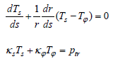
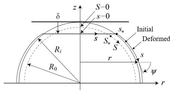
A computational model of a spherical cell compressed by two parallel plates is shown in Figure 1. The deformation is assumed to be axisymmetric, and only the upper half is treated assuming the vertical symmetry of the shape. The initial radius of the cell is denoted as Ri, and the displacement of the upper half when it is compressed by the plate is denoted as δ. The cytoskeleton consists of actin filaments, microtubules, and intermediate filaments. The actin filaments, which exist along the inner side of the cell membrane, mainly support the mechanical structure of the surface [20]. Therefore, we modeled the cell surface as an elastic membrane. In addition, the actin filaments, microtubules, and intermediate filaments inside the cell support the structure of the whole cell [17]. Therefore, we represent the actions of these components as the maintenance of the original volume of the whole cell. Cells adhere to the plates during plate compression, and in general, membrane tension is generated when cells adhere to a plate [21,22]. This tension is treated as the initial tension and modeled as follows. When there is no tension in the cell membrane, the cell is a sphere of radius R0, and the initial tension Ti is generated when the sphere expands to radius Ri. At this time, the initial stretch of the membrane is λi = Ri / R0 . The axis along the meridian of the sphere of radius R0 is denoted as S, and that along the meridian of the shape after deformation due to plate compression is denoted as s. The angle between axis s and axis r is denoted as ψ . For an axisymmetric elastic membrane, the equations of the static force balance in the tangential and normal directions in the meridian plane are given as follows [10], in which the bending stiffness of the membrane is ignored.
biomedres-openaccess-journal-bjstr

Figure 1: Analysis model.

Here, Ts and Tφ represent the principal tensions in the meridian plane and the principal tension in the circumferential direction, respectively. κ s and κϕ represent the principal curvature in the meridian plane and the principal curvature in the orthogonal plane, respectively. ptr represents the transmural pressure, i.e., the pressure difference between the inside and outside (internal pressure – external pressure). The principal stretch in the meridian plane λs and the circumferential principal stretch λφ are given by , where R represents the r coordinate in the initial state of the material point after deformation. The tensions Ts and Tφ are calculated using Evans and Skalak’s model [10] for biological membranes;


 , and Tφ is obtained by interchanging λs and λφ in Ts.

K(= Eh / 2(1− v)) represents the area-expansion modulus, and μ (= Eh / 2(1+ v)) represents the shear modulus. Here, E represents the Young’s modulus, h the membrane thickness, and ν the Poisson’s ratio. The isotropic tensions, i.e., the expansion tension Te, the shear tension Tsh, and the Mises tension TM, which is used to predict material failure according to the yield condition of the material, are determined using the following equations.

The Young’s modulus E and Poisson’s ratio ν are for membranes, but when determining the elastic modulus of a cell using atomic force microscopy, the Young’s modulus E’ of the entire cell is often determined using the relationship between the force and displacement for the entire cell. Therefore, the approximate relationship ' i Eh = E R for ν = 0.5 was used to obtain the Eh from E’ and Ri. The above equations were solved under the condition that the volume inside the cell does not change and the symmetry conditions of the shape at z = 0 (i.e.ψ = Ï€ /2) to determine the strain of the cell, deformation shape, tension distribution, and pressure difference for the compressive force. The calculation method was described in detail in [19].

Results and Discussion

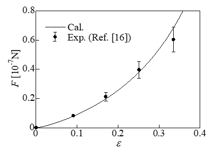
To validate the computational model, a comparison with experimental results (16) was performed. In this experiment, a single endothelial cell was subjected to a compression test using parallel plates, and the relationship between the force F and the compressive strain ε (= δ / Ri) was determined, as shown in Figure 2. In the calculation, the cell diameter was assumed to be 17.4μm, according to the experimental images. The Young’s modulus E’ of the whole cell was set as 1220Pa according to the Young’s modulus of the cytoplasm (1000Pa), the Young’s modulus of the nucleus (2500Pa), and the estimated volume ratio of the nucleus to the cytoplasm (0.17). Fitting to the experimental results was performed with the initial stretch set as λi = 1.12. The calculation results are indicated by the solid line in Figure 2. They agreed well with the experimental results with reasonable errors. According to the calculation, the initial tension determined from the initial stretch of the membrane was 2.7mN/m. According to measurements of HeLa cells (15-25μm in diameter) attached to a substrate, the membrane tension ranged from 2.73 to 3.62mN/m [22]. The results of the present calculations are close to these values.

biomedres-openaccess-journal-bjstr

Figure 2: Relationship between the force and compressive strain.

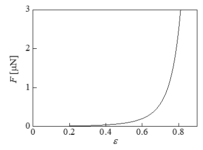
When cells are frozen at a low temperature drop rate, ice crystals develop in a needle-like shape on the outside of the cells over time, and the cells appear to be compressed in the narrow spaces between the crystals [7,8]. Therefore, Takamatsu, et al. [1] hypothesized that the mechanical stress of compression is a major cause of cell damage during cell freezing, and as a model experiment, they performed compression tests on cells using parallel plates and investigated the relationship between the compression rate and the cell viability. The target cells were human prostatic adenocarcinoma cells. In the experiment, the change in the cell size caused by the change in the external osmotic pressure generated during cell freezing was considered; i.e., compression testing was performed on these cells by changing the concentration of an extracellular NaCl aqueous solution, which changed the cell diameter to 15.4, 17.8, and 20.5μm. Table 1 presents the relationship between the compressive strain ε and the cell viability, which were averaged for the three kind of cells. The data were taken from Figure 6 in Ref. [1]. For the cell with diameter d (= 2Ri) = 17.8μm, calculations were performed for compression due to parallel plates. The Young’s modulus of the membrane E of prostate cancer was calculated using the measured Young’s modulus of a whole cell, i.e., E’ = 452Pa [23]. The initial stretch was set as λi = 1.12, which was used in the calculation shown in Figure 2. The calculation results for the relationship between the compressive force F and the strain ε are presented in Figure 3. When the strain was larger than ε = 0.7, the force F increased rapidly; thus, the viability decreased significantly, as shown in Table 1.

biomedres-openaccess-journal-bjstr

Table 1: Relationship between the compressive strain and the cell viability [1].

biomedres-openaccess-journal-bjstr

Figure 3: Relationship between the compressive force and the strain (d = 17.8μm).

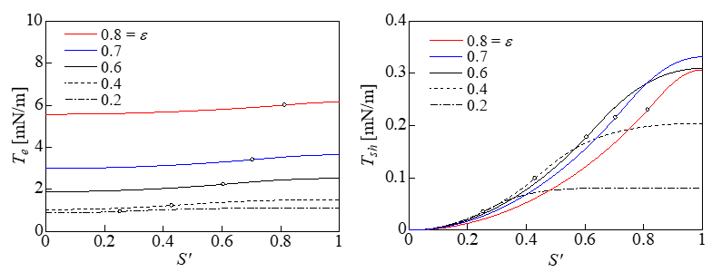
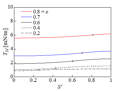
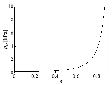
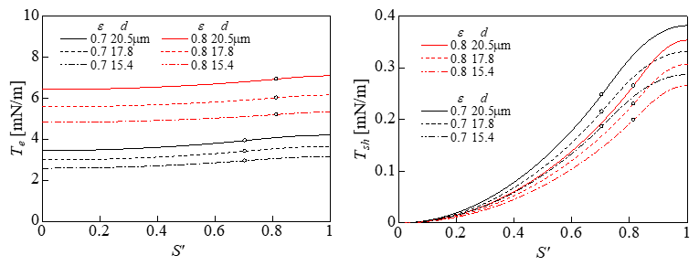
Figure 4 shows the variations in the expansion tension Te and shear tension Tsh with respect to the dimensionless S ' (= 2S /Ï€ R0 ) when the strain ε was varied. The white circles in the figure indicate the points corresponding to S*. The contact area with the plate is shown on the left of the white circles, and the non-contact area with the plate is shown on the right. Te was approximately uniform on the membrane and was maximized at S’ = 1 ; i.e., at z = 0. In addition, Te increased with the strain ε. The shear tension Tsh increased with S’ and was maximized at z = 0. However, Tsh was approximately one order of magnitude lower than Te. Figure 5 shows that the distribution of the Mises tension TM was almost identical to Te in Figure 4, indicating that the expansion tension caused cell lysis. Figure 6 shows the relationship between the strain and the pressure difference. When a cell lyses, the pressure difference is thought to decrease to zero from the pressure difference immediately before the lysis. The volume loss during compression is derived from dV = ALp ptrdt , where Lp is the water permeability of the cell membrane. The value for the erythrocyte membrane Lp = 0.92 × 10- 12m/sPa [24] was used as Lp, the surface area of a spherical cell of diameter 17.8μm was used as the surface area A, and dt represents the time (10min) that the cell was under compression [1]. The rates of volume loss were 19% and 37% at ptr = 1 and 2 kPa, respectively. In this cell model, the cytoskeleton inside the cell works to keep the volume of the whole cell constant, and the water permeability of the membrane is ignored.

biomedres-openaccess-journal-bjstr

Figure 4: Variations in Te and Tsh (d = 17.8μm).

biomedres-openaccess-journal-bjstr

Figure 5: Variations in TM (d = 17.8μm).

biomedres-openaccess-journal-bjstr

Figure 6: Relationship between the pressure difference and the strain (d = 17.8μm).

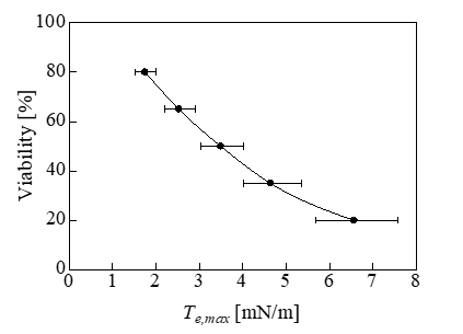
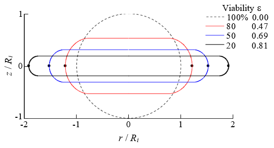
To investigate the effect of the change in the cell diameter on the tension, we performed calculations for cells with diameters of 15.4, 17.8, and 20.5μm with ε = 0.7 and 0.8. The calculation results for Te and Tsh are shown in Figure 7. Te and Tsh both increased with the diameter. Therefore, it was expected that a larger diameter would correspond to lower cell viability, similar to the results of a previous experiment [1]. Figure 8 shows the relationship between the maximum value of Te, i.e., Te,max, and the viability of cells with a diameter of 17.8μm. The error bars in Figure 8 indicate the changes in Te,max when the diameter changed from 15.4 to 20.5μm. The causal factor triggering the cell lysis was thought to be the Te,max in Figure 8. The positions of Te,max are indicated by the black dots in Figure 11. The cytoskeletal structure of erythrocytes is mainly composed of spectrin on the inner side of the cell membrane, which differs from the cytoskeletal structure of prostatic adenocarcinoma cells. The expansion tension at which erythrocytes undergo hemolysis is Th = 15mN/m [25], which exceeds the maximum value (Te,max) in Figure 8. The radius of the erythrocyte when it was expanded to a sphere without changing the surface area from its initial value of 138μm2 [26] was assumed to be rh. The pressure difference ptr at this time was ptr = 9.1 kPa calculated by the Laplace equation ptr = 2Th / rh . This was the pressure difference that causes hemolysis of erythrocytes. By comparing this value with the results shown in Figure 6, the compressive strain was determined to be 0. 87.

biomedres-openaccess-journal-bjstr

Figure 7: Changes in Te and Tsh.

biomedres-openaccess-journal-bjstr

Figure 8: Relationship between the maximum expansion tension and the cell viability.

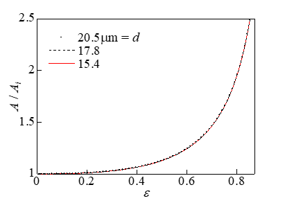
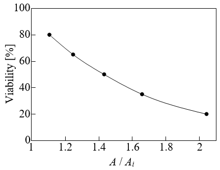
The surface area increases when cells are compressed. The results of the effect of the change in the cell diameter on the rate of increase of the surface area A/Ai during compression are presented in Figure 9. Here, Ai (=π d 2 / 2) represents the surface area in the initial state. As shown in Figure 9, the effect of the change in the cell diameter on A/Ai was negligible. Therefore, the rate of increase of the surface area was independent of the cell size and was used as an evaluation index for the cell viability. Figure 10 shows the relationship between A/Ai and the viability. The results shown in Figures 9 & 10 are almost the same as those in Ref. [1]. Figure 11 shows the deformed shape of the cell resulting from compression. Here, ε = 0, 0.47, 0.69 and 0.81 correspond to the initial state and the compression states at 80%, 50%, and 20% viability, respectively. Because the deformation shape was independent of the cell diameter, a dimensionless representation with the initial radius Ri as the representative length is presented in Figure 11. Thus, the deformation shape was independent of the cell size and was used as an evaluation index for the cell viability. The black circle indicates the position where the expansion tension reached its maximum value Te,max.

biomedres-openaccess-journal-bjstr

Figure 9: Relationship between the strain and the rate of increase of the surface area.

biomedres-openaccess-journal-bjstr

Figure 10: Relationship between the rate of increase of the surface area and the cell viability.

biomedres-openaccess-journal-bjstr

Figure 11: Relationship between the dimensionless deformation shape resulting from compression and the cell viability.

Conclusion

We performed calculations to model the process of cells being compressed by the development of external ice crystals in cell freezing under a slow temperature drop and obtained the following results.

1) The cause of cell lysis was expansion tension in the membrane of cortical actin filaments, and the effect of shear tension was negligible.

2) When the cell size increased owing to external osmotic pressure, the expansion tension due to the compression increased. Therefore, larger cells had lower viability under compression.

3) For prostatic adenocarcinoma cells with a diameter of 17.8μm, the expansion tensions that resulted in 50% and 20% viability were 3.5 and 6.6mN/m, respectively, and the rates of increase in the surface area were 1.4 and 2.0, respectively. 4) The rate of increase of the surface area under compression and the deformation shape are indices of the cell viability, because they are independent of the cell size in the range from d =15.4 to 20.5μm.


For more Articles on: https://biomedres01.blogspot.com/

Wednesday, June 12, 2024

A New Quantitative Method for Detecting SNP Heterozygous Samples by Sanger First Generation DNA Sequencing


A New Quantitative Method for Detecting SNP Heterozygous Samples by Sanger First Generation DNA Sequencing

Introduction

Sanger DNA sequencing is the widely used “gold standard method” to verify the results of TaqMan qPCR and second generation DNA sequencing [1-5]. At the same time, with the technological and commercial advances, many outsourcing companies provide Sanger DNA sequencing services [6,7]: as long as the customer provide the sequencing materials and information, such as DNA template, amplification primers, sequencing primers, and sequencing requirements for the target DNA, the outsourcing companies can professionally perform the steps including the amplification of target DNA template fragments with ordinary PCR, electrophoresis, recovery of amplified DNA template fragments, mixing DNA templates, sequencing primers and sequencing dye mixture Big Dye, sequencing the DNA template on Sanger sequencer, and finally the DNA sequencing map is produced, which can be opened and analyzed by the open software Chromas.

SNP is the abbreviation of single nucleotide polymorphism. SNP exists widely in human genome [8,9]. For a specific SNP site, human beings have two sequence sources, one from father and the other from mother [10-12]. Therefore, for human SNP sites, there are homozygous and heterozygous genotypes: homozygous genotype refers to same SNP signals from father and mother, and heterozygous genotype refers to different SNP signals from father and mother. For the case of heterozygosity, the two SNP signals are usually equal in quantity, and the ratio is 1:1. The detection of heterozygous SNP samples is generally based on TaqMan PCR and second-generation DNA sequencing to find putative sites, and then further verified by Sanger DNA sequencing. Because the heterozygous SNP samples have different SNP signals of 1:1, there will be two overlapping signal peaks at the SNP sequencing map, so it can be judged that this person is heterozygous genotype for that SNP site. However, due to the process of DNA extraction or the existence of genomic chimerism in heterozygous SNP samples, the amount of two kinds of SNP signals is sometimes not 1:1, and there may be a variety of ratios such as 2:1, 5:1, 10:1, 20:1, etc. The sequencing maps for heterozygous SNP samples with those unconventional ratios have not been systematically studied, which will cause misjudgment or missed judgment.

In this study, we artificially simulated SNP heterozygous samples with nucleotides polymorphisms, mixed two of the DNA templates with different SNP in the ratio of 1:1, 2:1, 5:1, 10:1 and 20:1, and then analyzed the SNP sequencing map for the samples with different ratios, in order to establish the overlapping model map of nucleotide signals at different ratios, providing reference for correctly judging the SNP heterozygosity for different nucleotides.

Materials and Methods

DNA Templates and Primers for PCR and Sequencing DNA Templates:

(1) Template 1: P-ctDNA-1, the sequence is as follows, and the SNP site was heavily marked red: 5’-AGCAGAGGGGACATGAAATAGTTGTCCTAGCACCTGACGCCTCGT TGTACATCAGAGACAGAGCATTTT ACACCTTGAAGACGTACCCTG-3’;

(2) Template 2: P-ctDNA-2, the sequence is as follows, and the SNP site was heavily marked red: 5’-AGCAGAGGGGACATGAAATAGTTGTCCTAGCACCTGACGCCTCGTTGTACATCAGAGACGGAGCATTTT ACACCTTGAAGACGTACCCTG-3’;

(3) Template 3: P-ctDNA-C, the sequence is as follows, and the SNP site was heavily marked red: 5’-AGCAGAGGGGACATGAAATAGTTGTCCTAGCACCTGACGCCTCGT TGTACATCAGAGACCGAGCATTTT ACACCTTGAAGACGTACCCTG-3’;

(4) Template 4: P-ctDNA-T, the sequence is as follows, and the SNP site was heavily marked red: 5’-AGCAGAGGGGACATGAAATAGTTGTCCTAGCACCTGACGCCTCGT TGTACATCAGAGACTGAGCATTTT ACACCTTGAAGACGTACCCTG-3’;

(5) Preparation of SNP heterozygous sample templates: artificially mixed any two of P-ctDNA-1, P-ctDNA-2, P-ctDNA-C and P-ctDNA-T samples with the ratio of 1:1, 2:1, 5:1, 10:1 and 20:1, and the final concentration was 12 μM. PCR amplification primers: (1) Primer 1: forward primer, P-ctDNA-3: 5’-AGCAGAGGGGACATGAAATA- 3’;

(2) Primer 2: backward primer, P-ctDNA-4: 5’-CAGGGTACGTCTTCAAGGTG-3. Sequencing primer: P-ctDNA-3: 5’-AGCAGAGGGGACATGAAATA-3’.

Sequencing Outsourcing Services

Chengdu Branch of Nanjing Qingke Biotechnology Co., Ltd. (Qingke company) was selected as the sequencing service provider. All SNP heterozygous sample templates with different ratios, amplification primers and the sequencing primer, and sequencing requirements were provided to Qingke company. The target band size for sequencing was 90 base pairs. The sequencing operations were professionally carried out by Qingke company. Finally, we obtained the DNA sequencing maps, which were map files with suffix ab1.

Analysis of Sequencing Map

The software for sequencing map analyses was chromas 2.6.5, which is a freeware. The analysis method was as follows: using Chromas software to open the map file with suffix ab1, produce the map picture, focus on the picture details at the target SNP site, and eventually obtain the picture mode for the SNP heterozygosity.

Results

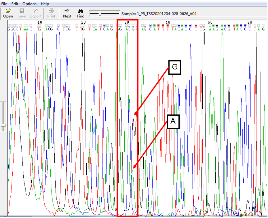
A: G = 1:1 in SNP Heterozygous Template

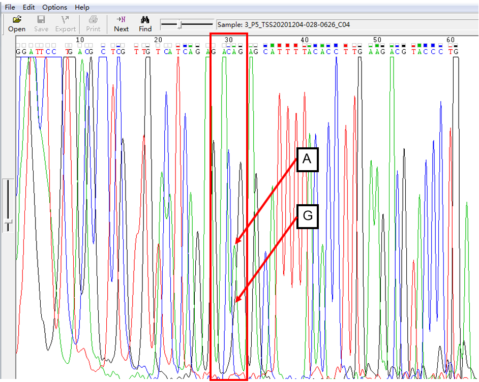
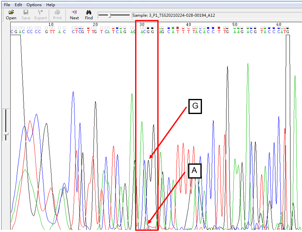
As shown in Figure 1, the signal of G overlapped with that of A, and the signal intensity of G was higher than that of A. This was the case of A: G = 1:1. The signal intensity is not only related to the amount of template, but also related to the fluorescent dye linked with different nucleotides.

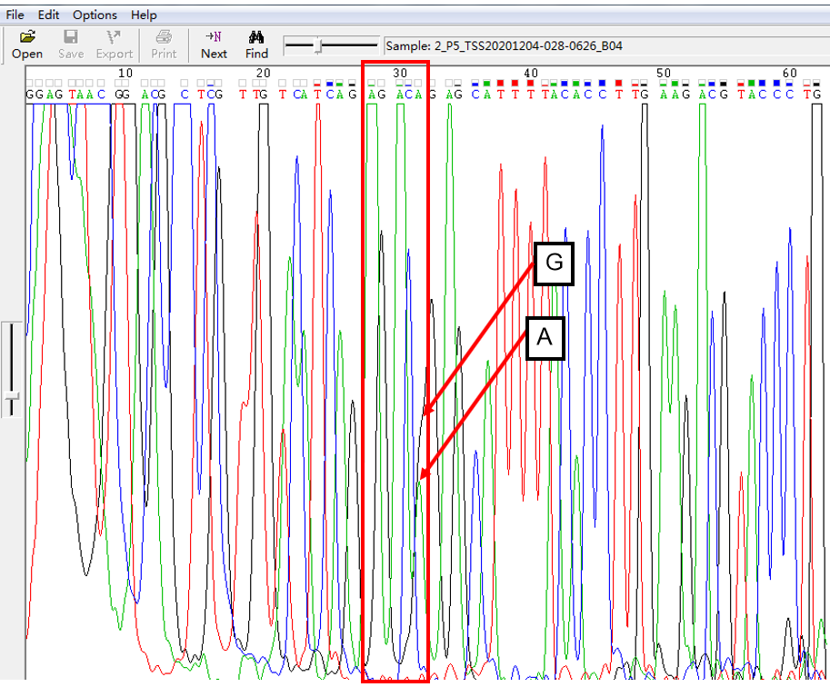
A: G = 2:1 in SNP Heterozygous Template

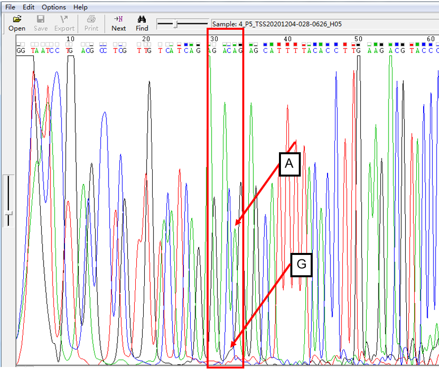
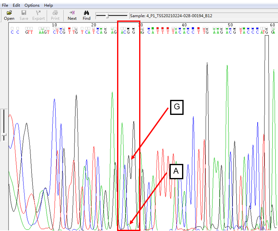
As shown in Figure 2, the signal of G overlapped with that of A, and the signal of G invaded the signal area of A in the form of a “big shoulder”. The signal intensity of G was higher than that of A, which was the case of A: G = 2:1.

A: G = 5:1 in SNP Heterozygous Template

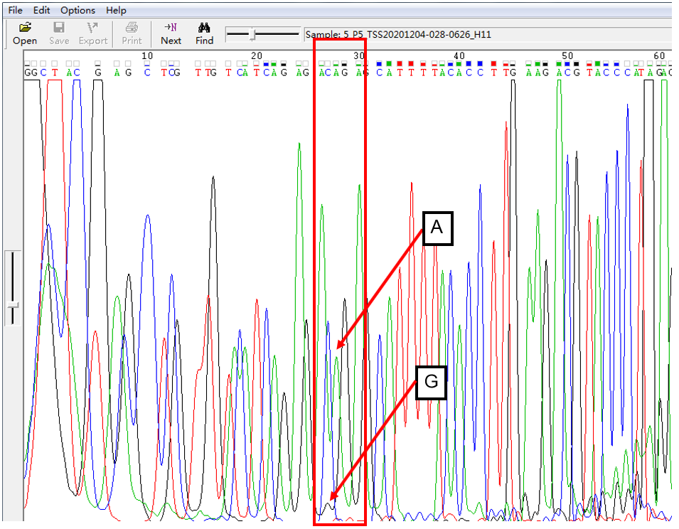
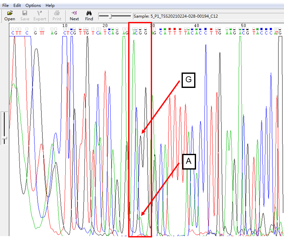
As shown in Figure 3, the signal of G overlapped with that of A, and the signal of G invaded into the signal area of A in the form of a “medium shoulder”. The signal intensity of G was lower than that of A, which was the case of A: G = 5:1.

biomedres-openaccess-journal-bjstr

Figure 1: The sequencing map of SNP heterozygous template when A: G = 1:1.

biomedres-openaccess-journal-bjstr

Figure 2: The sequencing map of SNP heterozygous template when A: G = 2:1.

biomedres-openaccess-journal-bjstr

Figure 3: The sequencing map of SNP heterozygous template when A: G = 5:1.

A: G = 10:1 in SNP Heterozygous Template

As shown in Figure 4, the signal of G overlapped with that of A, and the signal of G invaded into the signal region of A in the form of a “small shoulder”. The signal intensity of G was lower than that of A, which was the case of A: G = 10:1.

A: G = 20:1 in SNP Heterozygous Template

As shown in Figure 5, the signal of G overlapped with that of A, and the signal of G invaded into the signal region of A in the form of a “small shoulder”. The signal intensity of G was lower than that of A, which was the case of A: G = 20:1.

G: A = 2:1 in SNP Heterozygous Template

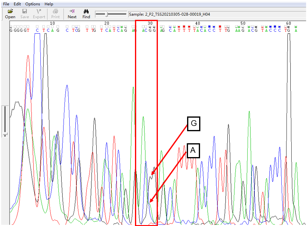
As shown in Figure 6, the signal of G overlapped with that of A, and the signal of A invaded the signal area of G in the form of a “big shoulder”. The signal intensity of G was higher than that of A, which was the case of G: A = 2:1.

G: A = 5:1 in SNP Heterozygous Template

As shown in Figure 7, the signal of G overlapped with that of A, and the signal of A invaded the signal area of G in the form of a “small shoulder”. The signal intensity of G was much higher than that of A, which was the case of G: A = 5:1.

G: A = 10:1 in SNP Heterozygous Template

As shown in Figure 8, the signal of G overlapped with that of A, and the signal of A invaded the signal area of G in the form of a “small shoulder”. The signal intensity of G was much higher than that of A, which was the case of G: A = 10:1.

G: A = 20:1 in SNP Heterozygous Template

As shown in Figure 9, the signal of G overlapped with that of A, and the signal of A invaded the signal area of G in the form of a “small shoulder”. The signal intensity of G was much higher than that of A, which was the case of G: A = 20:1.

biomedres-openaccess-journal-bjstr

Figure 4: The sequencing map of SNP heterozygous template when A: G = 10:1.

biomedres-openaccess-journal-bjstr

Figure 5: The sequencing map of SNP heterozygous template when A: G = 20:1.

biomedres-openaccess-journal-bjstr

Figure 6: The sequencing map of SNP heterozygous template when G: A = 2:1.

biomedres-openaccess-journal-bjstr

Figure 7: The sequencing map of SNP heterozygous template when G: A = 5:1.

biomedres-openaccess-journal-bjstr

Figure 8: The sequencing map of SNP heterozygous template when G: A = 10:1.

biomedres-openaccess-journal-bjstr

Figure 9: The sequencing map of SNP heterozygous template when G: A = 20:1.

Other SNP Heterozygous Templates

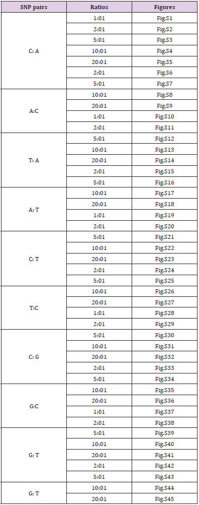
There were other pairs for SNP heterozygous templates summarized in the following Table 1 and supplementary materials.

biomedres-openaccess-journal-bjstr

Table 1: The summary of other pairs for SNP heterozygous templates.

Note: *p < 0.05 against CC, ^p < 0.05 against Post-HB, #p < 0.05 against Pre-HB.

Discussion

Through the analyses of SNP heterozygous samples with different proportions of samples, we could know the patterns of SNP heterozygous signals of different bases with various specific proportions, which could provide a judgment mode for using Sanger first generation DNA sequencing to verify SNP heterozygosity, which has not been systematically reported by all parties, so this study had the novelty. In conclusion, a new semi quantitative method for detecting SNP heterozygous samples solely by Sanger first generation DNA sequencing technology was established. This method can be used to guide the analysis of SNP heterozygous samples and is also suitable for the situation of limited data and the need for rapid SNP judgment in emergency.


For more Articles on: https://biomedres01.blogspot.com/
Antimalarial Aloe Compounds

  Antimalarial Aloe Compounds Introduction Among the most prevalent diseases caused by protozoan parasites, malaria is caused by parasites o...